


Abstract
This article brings control theory to life. Too often control theory is taught using block diagrams with no reference to real-life circuitry. With the help of some math and a circuit simulator, it can be shown that electronic control theory has relevance in modern electronic circuit design.
Introduction
Many subjects are taught in university that solicit the response from the student: “Will this get me a job?” Control theory might well be one of those subjects with no immediate use for pages of math and block diagrams of feedback systems. However, control theory teaches the engineer how to design systems that behave themselves, how close to the boundaries of stable operation a system is, and how to get the best response from any given system. Whether the subject is mechanical, electrical, civil, aeronautical, or communications engineering, if a system is not stable, it is of no use in the real world.
To the design engineer, control theory is life itself.
There are many excellent texts written on control theory, but many of them take a generalist approach, illustrated by block diagrams. This article is written for the electronics engineer and introduces electronic control theory from the viewpoint of circuit analysis and simulation. It explains the theory behind general second-order systems but illustrates the theory with worked circuit examples. The aim is to demystify the basics of second-order systems and explain to anyone trying to learn electronic control theory that it has relevance in analogue circuit design.
Second-order systems
The most basic second-order network is shown in Figure 1.
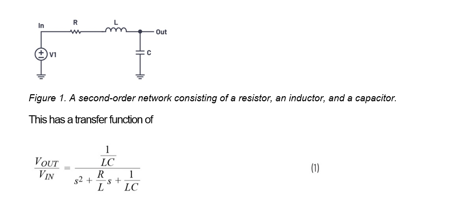
The denominator of the right hand side of Equation 1 is known as the characteristic polynomial and if we equate the characteristic polynomial to zero, we get the characteristic equation. The poles of a system occur when the denominator of its transfer function equals zero. By finding the roots of the characteristic equation (the values of s that make the characteristic equation equal to zero), we can find the poles of the system and hence discover a wealth of information about how the system behaves.
The general form of a second-order system transfer function is given by:
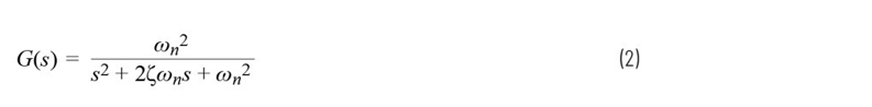
Where ζ is the damping coefficient and ωn is the circuit’s natural frequency (or undamped frequency) of oscillation in radians per second.
Therefore, the general characteristic equation for a second-order system is given by:
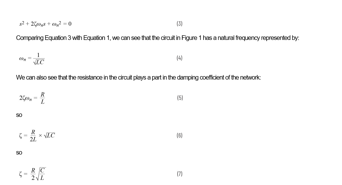
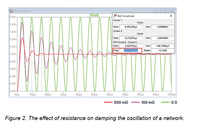
This is intuitive – if the circuit has no resistance, there is no loss in the network (no damping), so if the circuit is stimulated, it will oscillate forever. As resistance is increased, the oscillation decays more rapidly.
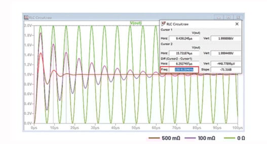
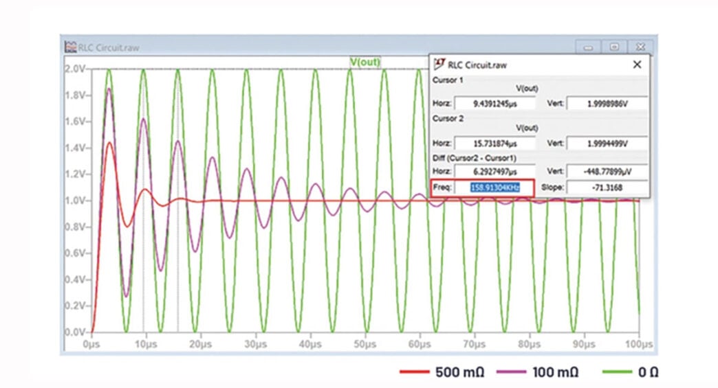
Figure 2 shows an RLC circuit excited with a 1V step input with values L = 1µH and C = 1µF, and resistances of 0Ω, 100mΩ, and 500mΩ. The circuit oscillates at a frequency of 159kHz, as expected. The effect of increased resistance on decay is clear.
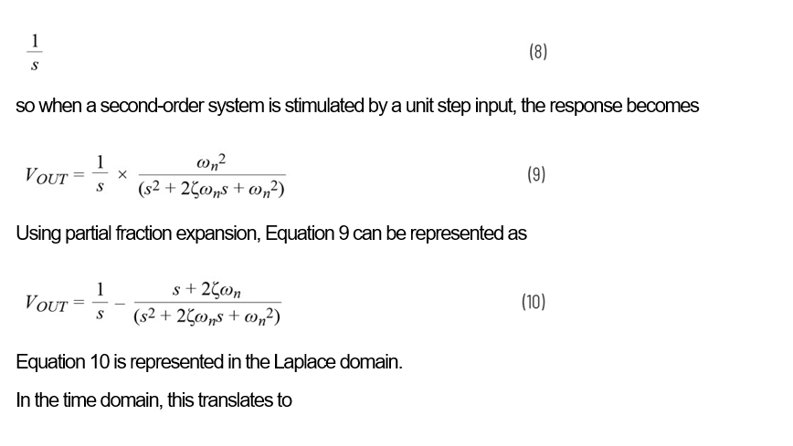
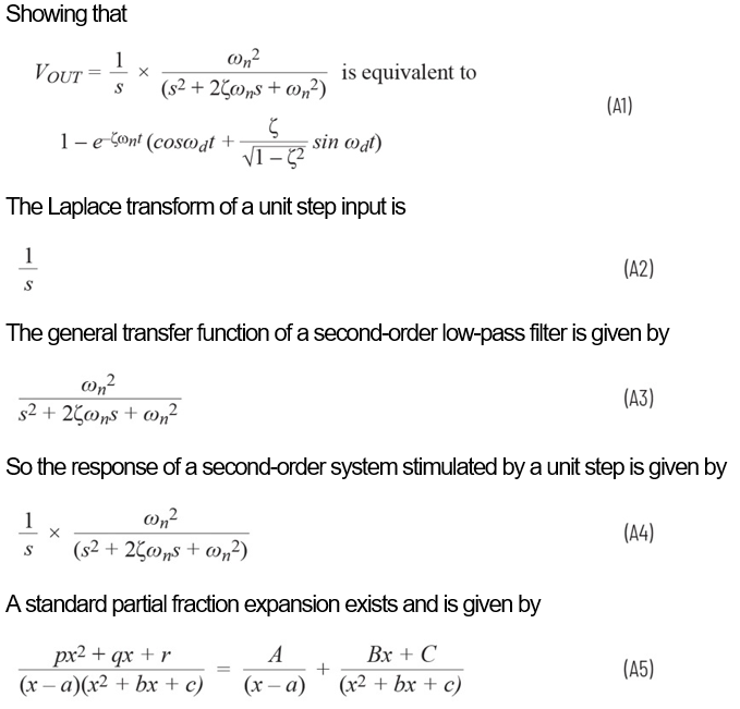
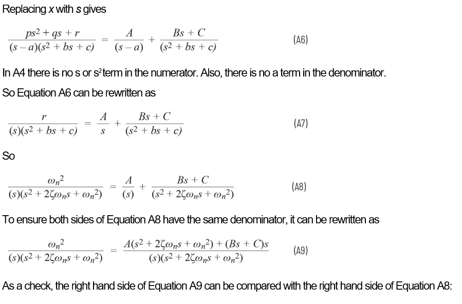
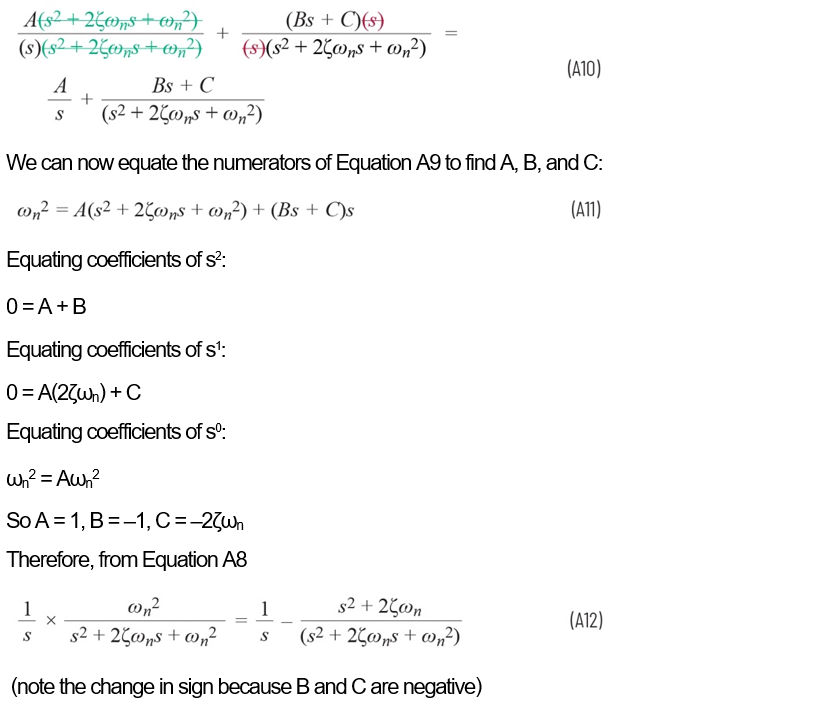
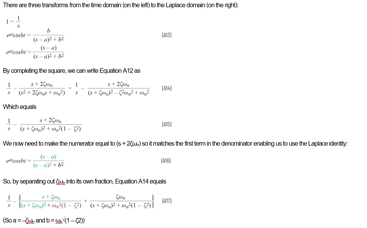
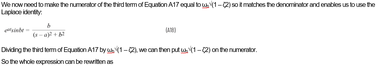
The results of the simulation shown in Figure 2 can be shown mathematically by translating from the Laplace domain to the time domain. A unit step input in the Laplace domain is represented by:
A mathematical derivation of Equation 11 with an inverse Laplace transform is shown in Appendix A.
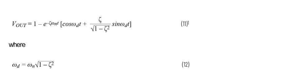
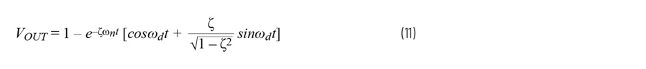
Equation 11 tells us how the circuit in Figure 1 responds to a step input. We can see that the waveform has a sinusoidal-like nature and its amplitude is modulated by the term e–ζωnt, which decays or grows exponentially depending on whether the damping coefficient is positive or negative. As an approximation, we can see that the response consists of a sinusoidal part and a cosinusoidal part, but, for low damping coefficients, the sinusoidal part is small.
Moreover, we can see that, although the natural frequency of the circuit is ωn, the circuit does not oscillate at this frequency but rather a frequency, ωd, that is somewhat lower and determined by the damping coefficient, ζ. This frequency is known as the damped natural frequency. Nevertheless, the exponential decay is dependent on the undamped natural frequency of the circuit, ωn.
The poles of a transfer function are found by determining when the denominator of the transfer function is equal to zero, namely:
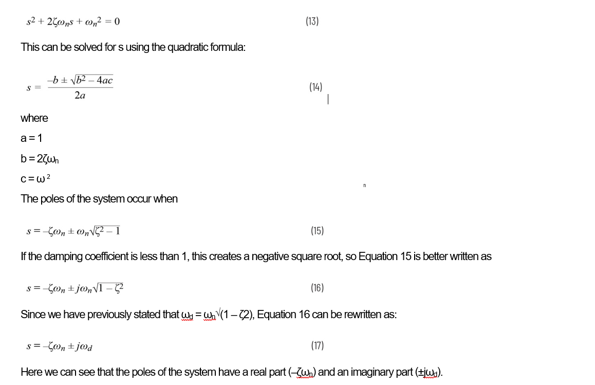
Here we can see that the poles of the system have a real part (–ζωn) and an imaginary part (±jωd).
Equation 17 tells us about the roots of the characteristic equation (the poles of the system). How can we relate these poles to the stability of the system? We now need to link the poles in the Laplace domain to the stability in the time domain.
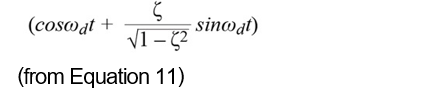
From Equation 11 and Equation 17, we can make the following observations. The undamped natural frequency, ωn, determines:
- The real part of the poles (–ζωn) in the Laplace domain (from Equation 17)
- The exponential decay in the time domain (e–ζωnt) (from Equation 11)
From this, it is reasonable to assume that the real part of the poles determines the exponential decay of the system.
The damped natural frequency, ωd, determines:
- The imaginary part of the poles (±jωd) in the Laplace domain (from Equation 17)
- The actual frequency of oscillation
From this, it is reasonable to assume that the imaginary part of the poles determines the actual frequency of oscillation of the system.
These two assumptions can be represented graphically in an s plane plot, which is discussed in the following section.
Stable systems
Control theory states that a system is stable if the poles lie in the left half of the s plane. Figure 3 shows an example of the s plane where the real part is plotted on the x-axis and the imaginary part is plotted on the y-axis.
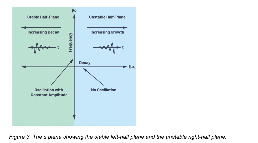
From Equation 17, we see that the poles lie in the left-half plane if the damping coefficient is positive (the real part of Equation 17 is negative). As the damping coefficient increases, the poles of Equation 17 move further to the left (further inside the left-half s plane).
If Equation 17 is in the Laplace domain, how does this translate in the time domain?
Equation 11 is repeated for convenience:
A positive damping coefficient, ζ, causes an exponentially decaying amplitude response (dictated by the term e–ζωnt) – the larger the damping, the quicker the decay. An increase in the damping coefficient moves the pole further inside the left-half s plane (in the Laplace domain), which increases the exponential decay in the time domain. This can be seen in Figure 2 with the 100mΩ and 500mΩ traces illustrating the effect of resistance on damping. The 500mΩ trace features the largest damping coefficient in this data, so its exponential decay is pronounced. At 0Ω, the damping coefficient is zero, where the poles lie exactly along the y-axis and the circuit oscillates indefinitely, as seen in the green trace in Figure 2.
It is worth noting that, although a system is stable, it is not necessarily without any oscillation. The circuit might be oscillatory with poles in the left-half plane, but the amplitude of these oscillations decay over time, as seen in Figure 2.
What does this mean for the circuit in Figure 1?
We know that the damping of Figure 1 is given by:
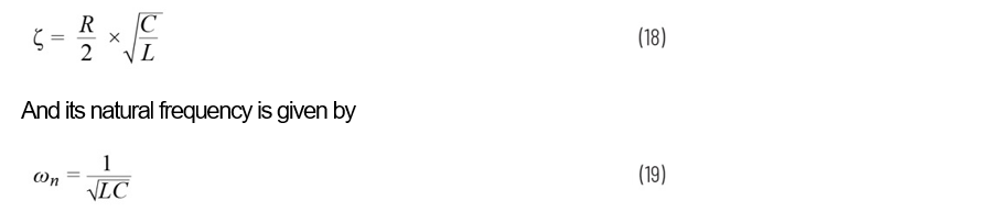
Therefore, with L = 1µH and C = 1µF, the natural frequency is 1Mrads–1 (= 159.1kHz) and the damping coefficient is 0.25 for R = 500mΩ.
Therefore, the damped oscillation frequency, ωd, is given by:

So, the damped oscillation frequency is 968krads–1, which is 154kHz. This is illustrated by looking at the frequency of the red waveform in Figure 4.
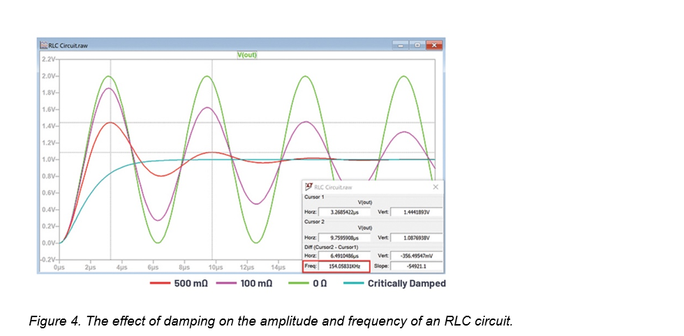
The amplitude of the sine wave decays by e–ζωnt. With a damping coefficient of 0.25, a natural frequency, ωn, of 1Mrads–1, and a damped natural frequency of 968246rads–1, Equation 11 becomes:

Using this formula, VOUT calculates to 1.44V at 3.26μs and 1.09V at 9.75μs, identical to the readings that can be seen in Figure 4.
Figure 4 clearly shows the effect of increasing the damping coefficient. Both the amplitude and the damped natural frequency reduce.
What happens if we keep increasing the damping coefficient?
We know that the damped natural frequency is given by:
![]()
We can see that if the damping coefficient is increased to unity, the damped natural frequency reduces to zero. This is known as the point of critical damping, where all oscillation in the circuit stops. This can also be seen in Equation 11. Since the damped natural frequency, ωd, has reduced to zero, the sine term equates to zero, the cosine term equates to unity, and the expression simplifies to a first-order system – identical to a capacitor charging through a resistor.

This can be seen in the critically damped trace in Figure 4.
Unstable systems
Since all circuits possess resistance, many electronic control circuits are inherently stable with poles lying in the left-half plane. However, from Equation 11, a negative damping coefficient causes an exponentially growing amplitude response, so poles lying in the right-half plane cause instability. With circuit simulation, it is easy to see the effect of a right-half plane pole by inserting a negative resistance. Figure 5 shows an RLC circuit, but where the resistance is negative.
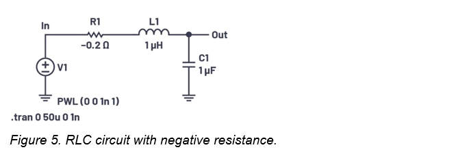
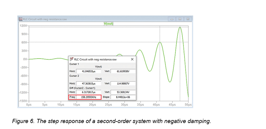
In this circuit, the damping coefficient is –0.1. Figure 6 shows its response to a step input.
The damped natural frequency is still dictated by:

And, for a damping coefficient of –0.1, the actual frequency of oscillation is 994987rads–1 (158.3kHz).
Again, from Equation 11, the response of our circuit is dictated by:

We can work out the amplitude response as the output grows: VOUT calculates to
61.62V at 41.05μs and to 114.99V at 47.36μs, which is identical to the readings shown in Figure 6.
Dominant poles
Sometimes a system consists of many poles, making analysis complicated. However, if the poles are spaced sufficiently apart, the effect of one pole often dominates the others and the system can be simplified by ignoring the non-dominant poles.
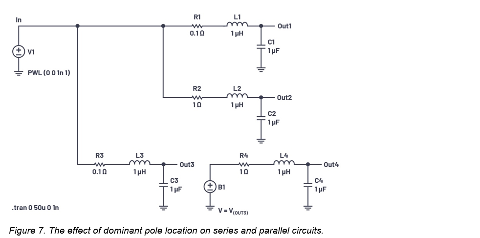
The top half of Figure 7 shows two RLC circuits, each with identical L and C components; only the resistance has been changed. The circuit with the lower resistance has its pole closer to the imaginary axis in the s plane.
The bottom half of Figure 7 shows these two circuits in series. V(OUT3) has been replicated using a behavioural voltage source, B1, to avoid it being loaded with R4, L4, and C4 so we can see the true response of V(OUT3) × V(OUT4).
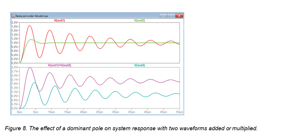
We can see their responses in Figure 8. Unsurprisingly, the circuit with the largest resistance has the largest damping coefficient, hence its oscillation decays the quickest, as seen in the plot of V(OUT2). However, we notice that when both outputs are either added (putting the circuits in parallel), or multiplied (putting the circuits in series), V(OUT1) dominates the response. Therefore, one way to simplify a complex system is to focus on the circuit that has poles closer to the jω axis, which tends to dominate the system response.
Systems with poles in both left- and rRight-half planes
We have considered systems with poles in either the left- or the right-half plane. What happens if the system has poles in both the left- and right-half planes? Which one wins the battle for stability and why?
Referring again to Equation 11, it is the exponent that determines if the system is stable. We can ignore the sinusoidal part of Equation 11 and just look at the exponents to see what happens if we combine a left-half pole with a right-half pole. Figure 9 shows a simple circuit to demonstrate this.
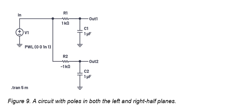
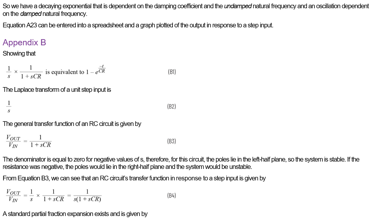
The RC circuit at the top clearly has a left-half pole since its resistance is positive. The circuit at the bottom has a right-half pole. A mathematical derivation of this is shown in Appendix B.
The response of the circuit in Figure 9 is shown in Figure 10.
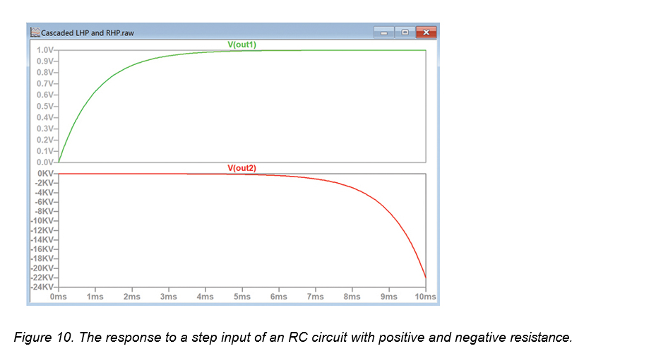
The top waveform settles to a zero gradient after about 5ms, matching the generally accepted rule that an RC circuit will settle in about five time constants. In contrast, V(OUT2) shows an ever-increasing gradient. It should now be apparent that if a circuit with a left-half plane pole is connected in series with a circuit with a right-half plane pole, then the complete circuit will be unstable since the right-half plane response continues to exponentially increase long after the left-half plane circuit has settled. So, for a circuit to be stable, all poles must lie in the left-half plane.
Conclusion
This article connects the theoretical models used in electronic control theory with the practical world of the electronics engineer. Control systems are stable if all poles lie in the left-half plane due to the resistance (or damping) present in the system. Practically demonstrating the response of a system with a right-half plane pole can prove problematic since it requires modelling a negative resistance. However, computer simulation comes to the rescue, enabling us to demonstrate stable and unstable circuits by simply changing the polarity of the resistance.
Likewise, Laplace transforms rarely manage to break out of the classroom, but here they have proved invaluable in proving how second-order electronic systems work.
Appendix A
Addendum
Simulations were conducted in LTspice.
Download the LTspice® files related to this article.
To learn more about LTspice, please visit analog.com/ltspice.
References
1 Charles Phillips and Royce Harbor. Feedback Control Systems, 4th edition. Prentice Hall International, 1988.
Acknowledgements
Thank you to Dr. Maysam Abbod, Brunel University, London for proofreading the theory.
About the author
Simon Bramble graduated from Brunel University in London in 1991 with a degree in electrical engineering and electronics, specialising in analogue electronics and power. He has spent his career in analogue electronics and worked at Linear Technology (now part of Analog Devices). He can be reached at simon.bramble@analog.com.