Coaxial transmission line

A schematic coaxial transmission line is depicted below and widely used both commercially and industrially, especially in connectors.

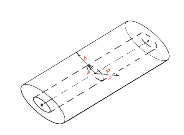
To obtain the field solution for a coaxial transmission line we have to resolve the Laplace equation for potential with the boundary conditions $\Psi (a)=V_0,\Psi (b)=0$. The easiest way to do this is to use polar coordinates similar to the ones used in a circular waveguide.

The potential function for a given type of coaxial waveguide is $\Psi (\rho ,\phi )=\frac{V_0\ln {\displaystyle \frac{b}{\rho }}}{in\frac{b}{a}}$. A coaxial line can perform TEM, TE and TM modes. However, in practice the TEM mode is the most common used mode.

Let’s consider the TE mode with $E_Z=0, H_Z\ne 0$, so we must resolve the Laplace equation for $H_Z$. The solution for $H_Z$ will be the following: $\mathrm{Hz}(\rho ,\phi )=(\mathrm{Asinn\phi }+\mathrm{Bcosn\phi })({\mathrm{CJ}}_n‘\; (k_c\rho )+{\mathrm{DY}}_n‘\; (k_c\rho ))e^{–\mathrm{j\beta z}}$, where $J$ and $Y$ are Bessel functions. The type of electric field function can be obtained using the boundary conditions. The cut-off number here will be $k_c=\frac{2}{a+b}, f_c=\frac{{\mathrm{ck}}_c}{2\pi \surd \epsilon }$.

The transmission line of parallel planes, stripes and microstripes