Fundamentals of power integrity measurement – part two
In part two of his article on power integrity measurement (view part one in the November issue of Electronic Specifier Design), Erik Babbé, Marketing Brand Manager for Oscilloscopes, Keysight Technologies, offers ten tips for better power supply measurement.
Controlling power supply noise is increasingly important as more designs incorporate microcontrollers and related circuitry whose function can be upset by supply transients. In the first of these two articles, we looked at some of the fundamentals of power integrity measurement, including some of the sources of noise, the measurement challenge, use of attenuation and some basics on applying FFT functions. In this article, we offer ten practical tips for improving your power supply measurements.
Choose the lowest noise oscilloscope measurement path
To have the best chance of measuring any noise riding on your DC power supply, try to minimise the noise of your oscilloscope measurement system.
For many oscilloscopes the 50ohm input has less noise than the 1Mohm input. It is useful to take a null measurement on your complete oscilloscope measurement system, including the probe, to check it is appropriate for the power supply noise measurements you want to make. To make a null measurement, configure your oscilloscope and probes as you intend to use them, then short the input to ground (or short the inputs together on a differential probe) and measure the noise.
Limit bandwidth to cut measurement system noise
The noise voltage of an oscilloscope and probe is a function of frequency. Limiting the bandwidth used to that necessary for the measurement cuts the amount of oscilloscope and probe noise that shows up in the measurement. For example, on a Keysight MSOS804A oscilloscope (8GHz, 10bit ADC, 20GSample/s) with a N7020A power rail probe (2GHz, 1:1 attenuation), the null measure noise at a 2GHz measurement bandwidth is 1,040μV, compared to 460μV at a measurement bandwidth of 20MHz.
Use the least attenuation you can to cut measurement system noise
Oscilloscope probes come in a variety of attenuation ratios, including the widely used 10:1 passive probe that enables the measurement of signals that would otherwise exceed that maximum input to the scope. The downside of using attenuation is that the ratio of scope noise to signal increases proportional to the attenuation ratio.
For example, in a measurement of a 20MHz 50mV p-p sine wave with both a 10:1 probe and a 1:1 probe, the 1:1 measurement is 52mV p-p while the 10:1 measurement is 65mV p-p, a 25% overstatement caused by the reduced signal-to-noise ratio resulting from the higher attenuation ratio.
The best advice? Use the lowest attenuation ratio you can.
Use probe offset to increase dynamic range
Probe offset is a feature of active probes that enables the user to remove DC content from signals being measured, for example when measuring a small AC signal riding on a DC signal.
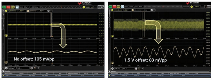
Figure 1. Measuring the noise on a 1.5VDC supply without (l) and with (r) probe offset.
Figure 1 shows the impact of applying probe offset, with the difference being due to the attenuation applied by the oscilloscope at the larger V/div settings.
It is worth remembering that most active probes that provide offset also have large attenuation ratios, which can make scope noise appear more significant than it is, as explained above.
Understand the limitations of DC blocks
A DC block is a specialised large value capacitor that can be placed in series with the signal to remove large DC components, so the scope can be placed in a more sensitive range. The limitation of a DC block is that it will also block low-frequency AC content, such as drift or supply compression. You can see the impact of this approach in Figure 2 (below).
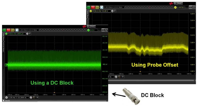
Figure 2: A DC block can mask low-frequency content, such as supply drift, in a way that using a probe offset does not in power supply noise measurements.
Using the DC block also means that DC measurements, such as the supply voltage, have to be made another way, for example with a multimeter.
Minimise oscilloscope and probe loading of the supply
When an oscilloscope probe is applied to a system, it changes the behaviour of the system being measured. It makes sense to minimise the loading that causes these changes, and in the case of measuring DC supplies, one common source of excessive loading is the use of a 50ohm coax between the supply and the scope. This makes sense in terms of using the low noise input and a shielded cable, but the scope will load the supply with 20mA/V, so that a 3.3V rail probed this way will experience a 66mA load from the oscilloscope.
A better approach is to use a probe such as the N7020A power-rail probe, which has a DC input impedance of 50Kohm. The supply was measured by a DMM and the probe at 3.31V, compared to 3.25V using the low impedance scope input and coax.
Use the frequency domain for analysis
Using an oscilloscope’s FFT capabilities to view signals in the frequency domain can help identify sources that contribute to the noise on a supply. In this example we have a switching DC/DC converter operating at 2.8MHz to convert 5V to 3.3V. The power supply PCB also carries 10MHz and 125MHz clock signals.
In this case, we are applying the previous tips and using the 1:1 attenuation ratio of a Keysight N7020A power rail probe, with 3.3V of probe offset and bandwidth limited to 500MHz to measure the noise on the 3.3V supply.
The probe is connected to a Keysight S-Series oscilloscope. Figure 3 shows the results of this measurement in the time domain, showing a signal of ~360ns period, the remnants of the 2.8MHz switching signal. What isn’t clear is the impact of the 10MHz and 125MHz clocks on the 3.3V supply.
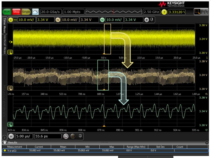
Figure 3: A time domain view of a 2.8MHz switching power supply, whose signal can be seen in the middle trace. The impact of nearby 10MHz and 125MHz clock signals aren’t obvious in the bottom, zoomed-in, trace.
Figure 4 shows the same data in the frequency domain. Using FFTs, we have set up windows covering two different frequency ranges, and we can clearly see a peak at 2.8MHz, which correlates with the switching frequency of the converter, and spikes at 10MHz and 125MHz, representing noise coupling in from the two clocks.
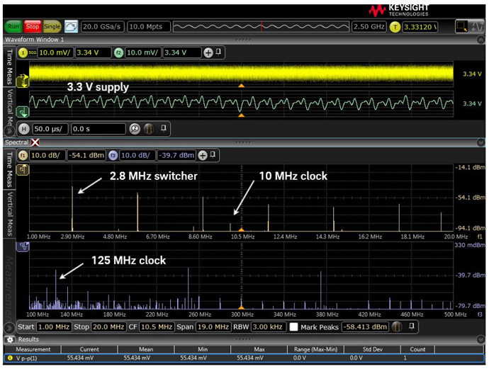
Figure 4: Using an FFT analysis to reveal noise from the 2.8 MHz switcher, and 10 MHz and 125 MHz clocks on the 3.3 V supply.
Use triggering to view and measure signal components in the supply noise
Another way of understanding a noise signal is to use triggering to reveal components of that noise that are coupling into the supply from other parts of the system.
Building on previous examples, imagine measuring a 2.8MHz switching regulator in a system with a 10MHz clock. Figure 4 shows the measurement results. The first step is to use an FFT to show that the 10 MHz clock is actually coupling into the power supply output. Once that is established we can trigger on that clock and turn on averaging to eliminate the random noise and other signal components that are not coherent with the clock. The end result is a trace of those portions of the supply noise that are correlated to the 10MHz clock, as shown in Figure 5.
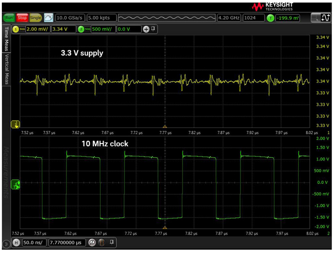
Figure 5: Triggering on the 10MHz clock and enabling averaging reveals the noise on the supply that is related to it.
Have enough bandwidth
Too much bandwidth can introduce unnecessary noise into your measurements, as we saw before. Too little bandwidth may mean missing high-frequency noise and transients that can affect clock and data signals. Switching currents from circuit features such as clocks, data lines and other sources can create supply noise that takes a measurement bandwidth of more than 1GHz to observe properly.
Consider using a N7020A power rail probe
Applying these tips should cut noise from the measurement system when trying to analyse power supply noise and identify its sources.
These techniques work even better when used with a dedicated power rail probe, such as the N7020A from Keysight Technologies. It has a 1:1 attenuation ratio, ±24V of offset, and connects to a scope’s 50ohm input. It also has 2GHz bandwidth to capture the high-frequency noise and transients that can cause clock and data jitter. Used with an oscilloscope such as the Keysight Infiniium S-Series, its bandwidth can be limited to reduce noise when its full 2GHz capability is not needed.
Product Spotlight
APV1111GVY
Panasonic
Panasonic PhotoMOS® Photovoltaic MOSFET High-Power Drivers
| SKU: | |
|---|---|
| Stock: | 3490 |
| Cost: | $3.95 |