A new approach to oscilloscope analysis
Debugging embedded systems often involves looking for clues that are hard to discover just by looking at one domain at a time. The ability to look at time and frequency domains simultaneously can offer important insights. Lee Morgan of Tektronix explains further.
Mixed domain analysis is especially useful for answering questions such as; what’s going on with my power rail voltage when I’m transmitting wireless data? Where are the emissions coming from every time I access memory? How long does it take for my PLL to stabilise after power-on?
Mixed domain analysis can help answer questions like these by providing views of time domain waveforms and frequency domain spectra in a synchronised view. Until now, the Tektronix MDO4000C mixed domain oscilloscope has been the only oscilloscope to offer synchronised time and frequency domain analysis with independent control over waveform and spectrum views. It accomplishes this by incorporating a full spectrum analyser with its own dedicated input channel.
To address the need for RF analysis in its 4, 5 and 6 Series MSO mixed signal oscilloscopes, Tektronix is taking a new approach that does not require a separate input channel while still offering similar capabilities. Recently released firmware unlocks an analysis tool called Spectrum View that takes advantage of patented hardware already in the instruments. With this tool, the scopes can now provide simultaneous analogue waveform views as shown on the left in Figure 1 and spectral views as shown on the right, with independent controls in each domain.
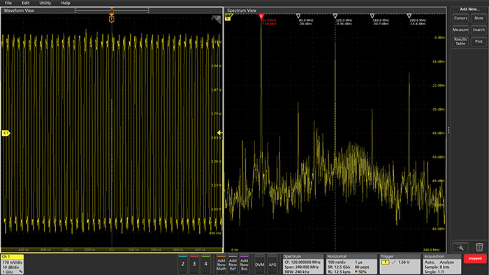
Figure 1. New firmware enables simultaneous analogue and spectrum views with independent controls in each domain
For more complex troubleshooting, instruments with the upgraded firmware can perform mixed domain analysis on more than one channel, as shown in Figure 2. Each of the two colour-coded analogue waveforms has a corresponding spectrum. Note that below each waveform is a small bar.
This indicates the time at which the spectrum occurs within the time domain. This spectrum time can be moved through the waveform to see the synchronised spectrum at any point in the waveform. In this example, the two channels show the startup of a clock signal from two different points in a circuit.
Oscilloscope analysis: scope FFTS vs. spectrum view
Although spectrum analysers are designed specifically for viewing signals in the frequency domain, they are not always readily available. Scopes, on the other hand, are almost always nearby in the lab so engineers tend to rely on scopes as much as possible. For this reason, oscilloscopes have included maths-based FFTs (fast fourier transforms) for decades. And most modern scopes let you look at amplitude-vs-time waveforms and amplitude-vs-frequency. So, what’s the big deal?
Let’s take a look. FFTs are notoriously difficult to use for two reasons. First, for frequency domain analysis spectrum analyser controls like centre frequency, span and resolution bandwidth (RBW) make it easy to define the spectrum of interest. In most cases, however, oscilloscope FFTs only support traditional controls such as sample rate, record length and time/div, making it difficult get to the right view.
Second, FFTs are driven by the same acquisition system as that used for the analogue time domain view. This means that speeding up the time scale in the time domain reduces resolution in the frequency domain. As a result, with conventional FFTs it’s virtually impossible to get optimised views in both domains. For example, in the screen shot in Figure 3 taken from a TDS3000, the time domain waveform is seen clearly, but FFT resolution is inadequate to see meaningful details.
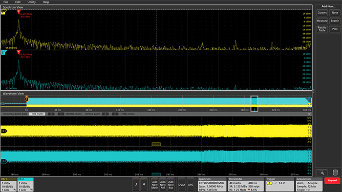
Figure 2. When debugging tasks demand it, multiple channels can be analysed simultaneously. Here, two channels show the startup of a clock signal from two different points in a circuit
In Figure 4, frequency modulation details are more visible with a slower time scale setting, but the time domain trace is now practically unusable.
In contrast, Spectrum View provides the ability to adjust the frequency domain using familiar centre frequency, span and RBW controls. And because these controls do not interact with the time domain scaling, it is possible to optimise both views independently as shown in Figure 5.
On-screen indicators (spectrum time) show the source of the spectrum on the waveforms. The ability to synchronise the two domains is useful for correlating signal activity on a board with EMI emissions, for example.
Conventional FFT trade-offs
The challenges with conventional FFTs go well beyond ease of use. To illustrate the performance tradeoffs engineers must consider, let’s say we have a tone at 900MHz and want to view its phase noise out to 50kHz on either side of the tone with 100Hz resolution. Ideally, the spectral view should have the following settings:
- Centre frequency: 900MHz
- Span: 100kHz
- RBW: 100Hz
With a traditional scope FFT, horizontal scale, sample rate and record length settings determine how the FFT works and must be considered holistically to produce the desired view.
Horizontal scale determines the total amount of time acquired. In the frequency domain, this determines your resolution. The more time you acquire, the better resolution you get in the frequency domain.
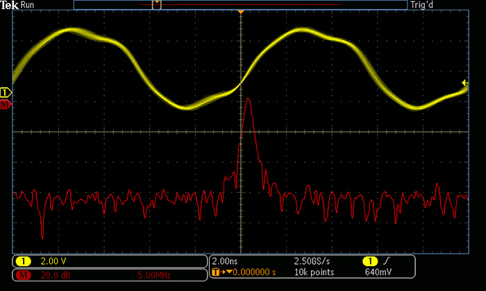
Figure 3. With the time domain optimised using conventional FFTs, frequency domain detail is lacking on this spread-spectrum clock signal
To resolve 100Hz, we need to acquire at least (1/100Hz) = 10ms of time. However, in reality we need to acquire nearly double that amount of time. In theory, FFTs are supposed to be applied to infinitely long signals. Since this isn’t possible, the beginning and end of the acquisitions introduce discontinuities (and thus error) into the resulting spectrum. To minimise discontinuities, the acquired record needs to fit in an FFT ‘window’. Most FFT windows have a bell or Gaussian shape where the ends are very low and the middle is high, meaning the spectrum must be primarily driven by the middle portion of the acquired data. Each window type has a constant associated with it. For this example, using a Blackman-Harris window type with a factor of 1.90 would require that we acquire 19ms (10ms*1.9 = 19ms) of time.
Sample rate determines the maximum frequency in the spectrum, where Fmax = SR/2. For a 900MHz signal, we need a sample rate of at least 1.8GS/s. Using the analogue sampling on the 5 Series as an example, we would sample at 3.125GS/s (first available sample rate above 1.8GS/s).
Now we can determine the record length. This is simply Time Acquired * Sample Rate. In this case, it’s 19ms * 3.125GS/s = 59.375 Mpoints record length.
Depending on the instrument, this record length may not even be available. Even if the scope has sufficient record length, many scopes limit the maximum length of an FFT because it is computationally intensive. For example, many previous generation oscilloscopes have a maximum FFT length of approximately 2Mpoints. Assuming you still want to see the 900MHz signal (which requires the high sample rate), you’d have to acquire approximately 1/30th of the desired time resulting in 30 times worse resolution in the frequency domain.
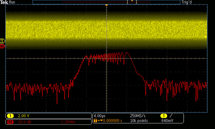
Figure 4. FFT tradeoffs are seen here with more frequency detail, but unusable time domain detail
As this example illustrates, setting up a desired view requires an appreciation of the complex interactions between horizontal scale, sample rate, and record length. Moreover, the reality of finite record length forces an undesirable compromise and observing high frequency signals with good resolution in the frequency domain requires extremely long data records which are often unavailable, or expensive and time consuming to process. Although some spectral analysis packages attempt to manage these trade-offs, all oscilloscope FFTs to date face the limitations described above.
Oscilloscope analysis: a new architecture
Giving users a way to perform spectral analysis without running into the inherent trade-offs of FFTs was a key design goal for Spectrum View. To understand how it works, it is important to note that digital oscilloscopes generally run their analogue-to-digital converters (ADC) at the maximum sample rate. The stream of ADC samples is then sent to a decimator that keeps every Nth sample. At the fastest sweep speeds, all samples are kept. At slower sweep speeds, it’s assumed the user is looking at slower signals and a fraction of the ADC samples are kept. In short, the purpose of the decimator is to keep the record length as small as possible while still providing an adequate sample rate to view signals of interest in the time domain.
In the 4, 5 and 6 Series MSOs, behind each FlexChannel input is a 12-bit ADC inside a custom ASIC called the TEK049. Each ADC sends high-speed digitised data down two paths. One path leads to hardware decimators which determine the rate at which time domain samples are stored.
The second path leads to digital down-converters (DDC) also implemented in hardware. This approach enables independent control of the time domain and frequency domain acquisitions, allowing optimisation of both waveform and spectrum views of a given signal. It also makes much more efficient use of the long but finite record length available in these instruments.
To illustrate the process, let’s consider the earlier 900MHz measurement scenario, but with the hardware digital down-converter added into the acquisition process.
The total time acquired still determines the resolution in the frequency domain. We also still need to apply an FFT window and acquire data for 19ms. In the TEK049, the ADC sends digitised time domain data to a decimator to create the time domain waveform view, but it also sends the data to the DDC.
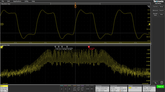
Figure 5. Looking at the same spread-spectrum clock signal as Figures 5 and 6, Spectrum View enables optimised views of both time and frequency domains on the same screen
As you might expect, the DDC has a profound effect on the required sample rate. The DDC shifts the centre frequency of interest from 900MHz to 0Hz. Now the 100kHz span goes from -50kHz to 50kHz. To adequately sample a 50kHz signal, we only need a sample rate of 125kS/s. Notice that by inserting the DDC into the acquisition process, the sample rate required becomes a function of span, not centre frequency.
Record length is governed by the same relationship as before. Record length is now 19ms * 125kS/s = 2,375 points. The data is stored as in-phase and quadrature (I&Q) samples and precise synchronisation is maintained between the time domain data and the I&Q data. Remember, in the case of a conventional FFT the required record length was 59.375Mpoints. The down-converted record only requires 2,375 points.
Now we perform an FFT on the 2,375 point I&Q record to get the desired spectrum. This dramatic reduction in the number of data points creates several important advantages:
- Update rate is greatly improved
- Much longer timespans can be processed and thus much better frequency resolution can be achieved in spectrum analysis
- The desired frequency domain view can be captured without changing the time domain view in any way
Oscilloscope analysis: toward more efficient system analysis
Efficient embedded system analysis and debugging begins and ends with insight. How can you possibly figure out why a system isn’t working as expected without precise, synchronised insight into both time and frequency domains? The answer is you can’t, and engineers have long recognised this, but they have been constrained by limitations in conventional oscilloscope FFTs.
A new oscilloscope architecture enabled by new firmware points the way to a number of significant advances:
- Enables the use of familiar spectrum analysis controls (Center Frequency, Span and RBW).
- Allows optimisation of both time domain and frequency domain displays independently.
- Enables a signal to be viewed in both a waveform view and a spectrum view without splitting the signal path.
- Enables accurate correlation of time domain events and frequency domain measurements (and vice versa).
- Significantly improves achievable frequency resolution in the frequency domain.
- Improves the update rate of the spectrum display.
Product Spotlight
APV1111GVY
Panasonic
Panasonic PhotoMOS® Photovoltaic MOSFET High-Power Drivers
| SKU: | |
|---|---|
| Stock: | 3490 |
| Cost: | $3.95 |